60 KiB
| author | title | lang | header-includes | abstract | documentclass | geometry | papersize | mainfont | fontsize | toc | nocite | ||||
|---|---|---|---|---|---|---|---|---|---|---|---|---|---|---|---|
| David Leppla-Weber | Search for excited quark states decaying to qW/qZ | en-GB | \usepackage[onehalfspacing]{setspace} \usepackage{siunitx} \usepackage{tikz-feynman} \usepackage{csquotes} \pagenumbering{gobble} \setlength{\parindent}{1.0em} \setlength{\parskip}{0.5em} \bibliographystyle{lucas_unsrt} | ```{=tex} Abstract. \end{abstract} \begin{abstract} Abstract 2. ``` | article |
|
a4 | Times New Roman | 12pt | true | @* |
\newpage \pagenumbering{arabic}
Introduction
The Standard Model is a very successful theory in describing most of the effects on a particle level. But it still has a lot of shortcomings that show that it isn't yet a full "theory of everything". To solve these shortcomings, lots of theories beyond the standard model exist that try to explain some of them.
One category of such theories is based on a composite quark model. They predict that quarks consist of particles unknown to us so far or can bind to other particles using unknown forces. This could explain some symmetries between particles and reduce the number of constants needed to explain the properties of the known particles. One common prediction of those theories are excited quark states. Those are quark states of higher energy that can decay to an unexcited quark under the emission of a boson. These decays are the topic of this thesis.
In previous research, a lower limit for the mass of an excited quark has already been set using data from the 2016 run
of the Large Hadron Collider with an integrated luminosity of \SI{35.92}{\per\femto\barn}. Since then, a lot more data
has been collected, totalling to \SI{137.19}{\per\femto\barn}. This thesis uses this new data as well as a new
technique to identify decays of highly boosted particles based on a deep neural network to further improve this limit
and therefore exclude the excited quark particle to even higher masses. It will also compare this new tagging technique
to an older tagger based on jet substructure studies used in the previous research.
First, a theoretical background will be presented explaining in short the Standard Model, its shortcomings and the theory of excited quarks. Then the Large Hadron Collider and the Compact Muon Solenoid, the detector that collected the data for this analysis, will be described. After that, the main analysis part follows, describing how the data was used to extract limits on the mass of the excited quark particle. At the very end, the results are presented and compared to previous research.
\newpage
Theoretical background
This chapter presents a short summary of the theoretical background relevant to this thesis. It first gives an introduction to the standard model itself and some of the issues it raises. It then goes on to explain the background processes of quantum chromodynamics and the theory of q*, which will be the main topic of this thesis.
Standard model
The Standard Model of physics proofed very successful in describing three of the four fundamental interactions currently known: the electromagnetic, weak and strong interaction. The fourth, gravity, could not yet be successfully included in this theory.
The Standard Model divides all particles into spin-\frac{n}{2} fermions and spin-n bosons, where n could be any
integer but so far is only known to be one for fermions and either one (gauge bosons) or zero (scalar bosons) for
bosons. The fermions are further divided into quarks and leptons. Each of those exists in six so called flavours.
Furthermore, quarks and leptons can also be divided into three generations, each of which contains two particles.
In the lepton category, each generation has one charged lepton and one neutrino, that has no charge. Also, the mass of
the neutrinos is not yet known, only an upper bound has been established. A full list of particles known to the
standard model can be found in [@fig:sm]. Furthermore, all fermions have an associated anti particle with reversed
charge. Multiple quarks can form bound states called hadrons (e.g. proton and neutron).

The gauge bosons, namely the photon, W^\pm bosons, Z^0 boson, and gluon, are mediators of the different
forces of the standard model.
The photon is responsible for the electromagnetic force and therefore interacts with all electrically charged particles. It itself carries no electromagnetic charge and has no mass. Possible interactions are either scattering or absorption. Photons of different energies can also be described as electromagnetic waves of different wavelengths.
The W^\pm and Z^0 bosons mediate the weak force. All quarks and leptons carry a flavour, which is a conserved value.
Only the weak interaction breaks this conservation, a quark or lepton can therefore, by interacting with a $W^\pm$
boson, change its flavour. The probabilities of this happening are determined by the Cabibbo-Kobayashi-Maskawa matrix:
\begin{equation} V_{CKM} = \begin{pmatrix} |V_{ud}| & |V_{us}| & |V_{ub}| \ |V_{cd}| & |V_{cs}| & |V_{cb}| \ |V_{td}| & |V_{ts}| & |V_{tb}| \end{pmatrix}
\begin{pmatrix}
  0.974 & 0.225 & 0.004 \\
  0.224 & 0.974 & 0.042 \\
  0.008 & 0.041 & 0.999
\end{pmatrix}
\end{equation}
The probability of a quark changing its flavour from i to j is given by the square of the absolute value of the
matrix element V_{ij}. It is easy to see, that the change of flavour in the same generation is way more likely than
any other flavour change.
The quantum chromodynamics (QCD) describe the strong interaction of particles. It applies to all particles carrying colour (e.g. quarks). The force is mediated by the gluon. This boson carries colour as well, although it doesn't carry only one colour but rather a combination of a colour and an anticolour, and can therefore interact with itself and exists in eight different variant. As a result of this, processes, where a gluon decays into two gluons are possible. Furthermore the strong force, binding to colour carrying particles, increases with their distance r making it at a certain point more energetically efficient to form a new quark - antiquark pair than separating the two particles even further. This effect is known as colour confinement. Due to this effect, colour carrying particles can't be observed directly, but rather form so called jets that cause hadronic showers in the detector. An effect called Hadronisation.
Quantum Chromodynamic background
In this thesis, a decay with two jets in the endstate will be analysed. Therefore it will be hard to distinguish the signal processes from QCD effects. Those can also produce two jets in the endstate, as can be seen in [@fig:qcdfeynman]. They are also happening very often in a proton proton collision, as it is happening in the Large Hadron Collider. This is caused by the structure of the proton. It not only consists of three quarks, called valence quarks, but also of a lot of quark-antiquark pairs connected by gluons, called the sea quarks, that exist due to the self interaction of the gluons binding the three valence quarks. Therefore in a proton - proton collision, interactions of gluons and quarks are the main processes causing a very strong QCD background.
\begin{figure} \centering \feynmandiagram [horizontal=v1 to v2] { q1 [particle=(q)] -- [fermion] v1 -- [gluon] g1 [particle=(g)], v1 -- [gluon] v2, q2 [particle=(q)] -- [fermion] v2 -- [gluon] g2 [particle=(g)], }; \feynmandiagram [horizontal=v1 to v2] { g1 [particle=(g)] -- [gluon] v1 -- [gluon] g2 [particle=(g)], v1 -- [gluon] v2, g3 [particle=(g)] -- [gluon] v2 -- [gluon] g4 [particle=(g)], }; \caption{Two examples of QCD processes resulting in two jets.} \label{fig:qcdfeynman} \end{figure}
Shortcomings of the Standard Model
While being very successful in describing mostly all of the effects we can observe in particle colliders so far, the Standard Model still has several shortcomings.
- Gravity: as already noted, the standard model doesn't include gravity as a force.
- Dark Matter: observations of the rotational velocity of galaxies can't be explained by the known matter. Dark matter currently is our best theory to explain those.
- Matter-antimatter assymetry: The amount of matter vastly outweights the amount of antimatter in the observable universe. This can't be explained by the standard model, which predicts a similar amount of matter and antimatter.
- Symmetries between particles: Why do exactly three generations of fermions exist? Why is the charge of a quark exactly one third of the charge of a lepton? How are the masses of the particles related? Those and more questions cannot be answered by the standard model.
- Hierarchy problem: The weak force is approximately
10^{24}times stronger than gravity and so far, there's no satisfactory explanation as to why that is.
Excited quark states
One category of theories that try to solve some of the shortcomings of the standard model are the composite quark
models. Those state, that quarks consist of some particles unknown to us so far. This could explain the symmetries
between the different fermions. A common prediction of those models are excited quark states (q*, q**, q***...).
Similar to atoms, that can be excited by the absorption of a photon and can then decay again under emission of a photon
with an energy corresponding to the excited state, those excited quark states could decay under the emission of some
boson. Quarks are smaller than 10^{-18} m, due to that, excited states have to be of very high energy. That will cause
the emitted boson to be highly boosted.
\begin{figure} \centering \feynmandiagram [large, horizontal=qs to v] { a -- qs -- b, qs -- [fermion, edge label=(q*)] v, q1 [particle=(q)] -- v -- w [particle=(W)], q2 [particle=(q)] -- w -- q3 [particle=(q)], }; \caption{Feynman diagram showing a possible decay of a q* particle to a W boson and a quark with the W boson also decaying to two quarks.} \label{fig:qsfeynman} \end{figure} This thesis will search data collected by the CMS in the years 2016, 2017 and 2018 for the single excited quark state q* which can decay to a quark and any boson. An example of a q* decaying to a quark and a W boson can be seen in [@fig:qsfeynman]. The boson quickly further decays into for example two quarks. Because the boson is highly boosted, those will be very close together and therefore appear to the detector as only one jet. This means that the decay of a q* particle will have two jets in the endstate (assuming the W/Z boson decays to two quarks) and will therefore be hard to distinguish from the QCD background described in [@sec:qcdbg].
To reconstruct the mass of the q* particle from an event successfully recognized to be the decay of such a particle,
the dijet invariant mass, the mass of the two jets in the final state, can be calculated by adding their four momenta,
vectors consisting of the energy and momentum of a particle, together. From the four momentum it's easy to derive the
mass by solving E=\sqrt{p^2 + m^2} for m.
\newpage
Experimental Setup
Following on, the experimental setup used to gather the data analysed in this thesis will be described.
Large Hadron Collider
The Large Hadron Collider is the world's largest and most powerful particle accelerator [@website]. It has a perimeter of 27 km and can collide protons at a centre of mass energy of 13 TeV. It is home to several experiments, the biggest of those are ATLAS and the Compact Muon Solenoid (CMS). Both are general-purpose detectors to investigate the particles that form during particle collisions.
Particle colliders are characterized by their luminosity L. It is a quantity to be able to calculate the number of
events per second generated in a collision by N_{event} = L\sigma_{event} with \sigma_{event} being the cross
section of the event. The luminosity of the LHC for a Gaussian beam distribution can be described as follows:
\begin{equation}
L = \frac{N_b^2 n_b f_{rev} \gamma_r}{4 \pi \epsilon_n \beta^}F
\end{equation}
Where N_b is the number of particles per bunch, n_b the number of bunches per beam, f_{rev} the revolution
frequency, \gamma_r the relativistic gamma factor, \epsilon_n the normalised transverse beam emittance, $\beta^$
the beta function at the collision point and F the geometric luminosity reduction factor due to the crossing angle at
the interaction point:
\begin{equation}
F = \left(1+\left( \frac{\theta_c\sigma_z}{2\sigma^*}\right)^2\right)^{-1/2}
\end{equation}
At the maximum luminosity of 10^{34}\si{\per\square\centi\metre\per\s}, N_b = 1.15 \cdot 10^{11}, n_b = 2808,
f_{rev} = \SI{11.2}{\kilo\Hz}, \beta^* = \SI{0.55}{\m}, \epsilon_n = \SI{3.75}{\micro\m} and F = 0.85.
To quantify the amount of data collected by one of the experiments at LHC, the integrated luminosity is introduced as
L_{int} = \int L dt.
Compact Muon Solenoid
The data used in this thesis was captured by the Compact Muon Solenoid (CMS). It is one of the biggest experiments at
the Large Hadron Collider. It can detect all elementary particles of the standard model except neutrinos. For that, it
has an onion like setup. The particles produced in a collision first go through a tracking system. They then pass an
electromegnetic as well as a hadronic calorimeter. This part is surrounded by a superconducting solenoid that generates
a magenetic field of 3.8 T. Outside of the solenoid are big muon chambers. In 2016 the CMS captured data of a integrated
luminosity of \SI{35.92}{\per\femto\barn}. In 2017 it collected \SI{41.53}{\per\femto\barn} and in 2018
\SI{59.74}{\per\femto\barn}. Therefore the combined dataset of all three years has a total integrated luminosity of
\SI{137.19}{\per\femto\barn}.
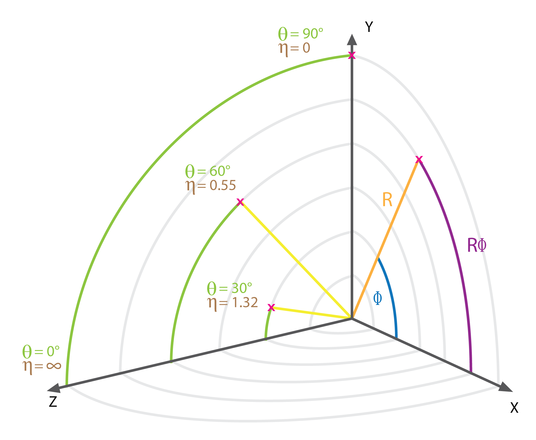
Coordinate conventions
Per convention, the z axis points along the beam axis, the y axis upwards and the x axis horizontal towards the LHC
centre. Furthermore, the azimuthal angle \phi, which describes the angle in the x - y plane, the polar angle \theta,
which describes the angle in the y - z plane and the pseudorapidity \eta, which is defined as $\eta =
-ln\left(tan\frac{\theta}{2}\right)$ are introduced. The coordinates are visualised in [@fig:cmscoords]. Furthermore,
to describe a particles momentum, often the transverse momentum, p_t is used. It is the component of the momentum
transversal to the beam axis. It is a useful quantity, because the sum of all transverse momenta has to be zero.
Missing transverse momentum implies particles that weren't detected such as neutrinos.
 {#fig:cmscoords width=60%}
The tracking system
The tracking system is built of two parts, first a pixel detector and then silicon strip sensors. It is used to reconstruct the tracks of charged particles, measuring their charge sign, direction and momentum. It is as close to the collision as possible to be able to identify secondary vertices.
The electromagnetic calorimeter
The electromagnetic calorimeter measures the energy of photons and electrons. It is made of tungstate crystal. When passed by particles, it produces light in proportion to the particle's energy. This light is measured by photodetectors that convert this scintillation light to an electrical signal. To measure a particles energy, it has to leave its whole energy in the ECAL, which is true for photons and electrons, but not for other particles such as hadrons and muons. They too leave some energy in the ECAL.
The hadronic calorimeter
The hadronic calorimeter (HCAL) is used to detect high energy hadronic particles. It surrounds the ECAL and is made of alternating layers of active and absorber material. While the absorber material with its high density causes the hadrons to shower, the active material then detects those showers and measures their energy, similar to how the ECAL works.
The solenoid
The solenoid, giving the detector its name, is one of the most important features. It creates a magnetic field of 3.8 T and therefore makes it possible to measure momentum of charged particles by bending their tracks.
The muon system
Outside of the solenoid there is only the muon system. It consists of three types of gas detectors, the drift tubes,
cathode strip chambers and resistive plate chambers. The system is divided into a barrel part and two endcaps. Together
they cover 0 < |\eta| < 2.4. The muons are the only detected particles, that can pass all the other systems
without a significant energy loss.
The Trigger system
The CMS features a two level trigger system. It is necessary because the detector is unable to process all the events due to limited bandwidth. The Level 1 trigger reduces the event rate from 40 MHz to 100 kHz, the software based High Level trigger is then able to further reduce the rate to 1 kHz. The Level 1 trigger uses the data from the electromagnetic and hadronic calorimeters as well as the muon chambers to decide whether to keep an event. The High Level trigger uses a streamlined version of the CMS offline reconstruction software for its decision making.
The Particle Flow algorithm
The particle flow algorithm is used to identify and reconstruct all the particles arising from the proton - proton collision by using all the information available from the different sub-detectors of the CMS. It does so by extrapolating the tracks through the different calorimeters and associating clusters they cross with them. The set of the track and its clusters is then no more used for the detection of other particles. This is first done for muons and then for charged hadrons, so a muon can't give rise to a wrongly identified charged hadron. Due to Bremsstrahlung photon emission, electrons are harder to reconstruct. For them a specific track reconstruction algorithm is used. After identifying charged hadrons, muons and electrons, all remaining clusters within the HCAL correspond to neutral hadrons and within ECAL to photons. If the list of particles and their corresponding deposits is established, it can be used to determine the particles four momenta. From that, the missing transverse energy can be calculated and tau particles can be reconstructed by their decay products.
Jet clustering
Because of the hadronisation it is not possible to uniquely identify the originating particle of a jet. Nonetheless,
several algorithms exist to help with this problem. The algorithm used in this thesis is the anti-k_t clustering
algorithm. It arises from a generalization of several other clustering algorithms, namely the k_t, Cambridge/Aachen
and SISCone clustering algorithms.
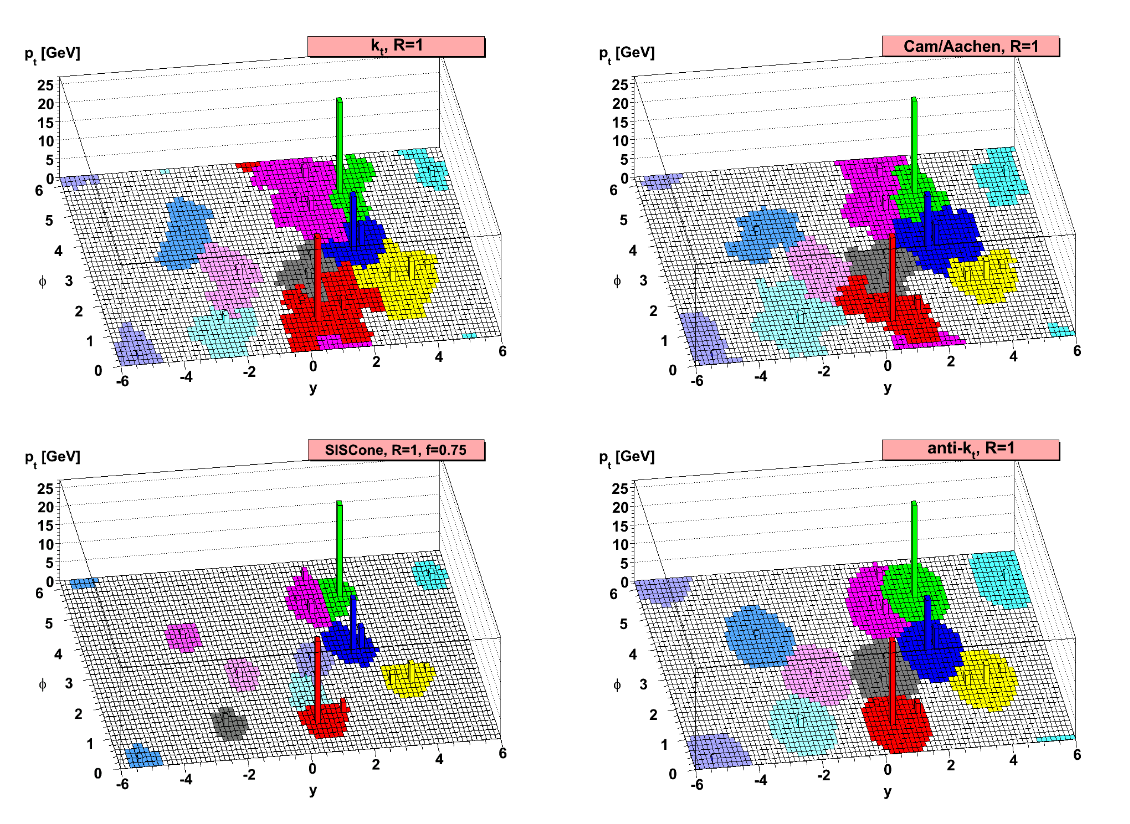
The anti-k_t clustering algorithm associates hard particles with their soft particles surrounding them within a radius
R in the \eta - \phi plane forming cone like jets. If two jets overlap, the jets shape is changed according to its
hardness. A softer particles jet will change its shape more than a harder particles. A visual comparison of four
different clustering algorithms can be seen in [@fig:antiktcomparision]. For this analysis, a radius of 0.8 is used.
Furthermore, to approximate the mass of a heavy particle that caused a jet, the softdropmass can be used. It is calculated by removing wide angle soft particles from the jet to counter the effects of contamination from initial state radiation, underlying event and multiple hadron scattering. It therefore is more accurate in determining the mass of a particle causing a jet than taking the mass of all constituent particles of the jet combined.
 {#fig:antiktcomparision}
\newpage
Method of analysis
This section gives an overview over how the data gathered by the LHC and CMS is going to be analysed to be able to either exclude the q* particle to even higher masses than already done or maybe confirm its existence.
- As described in [@sec:qs], an excited quark q* can decay to a quark and any boson. The branching ratios are calculated
- to be as follows [@QSTAR_THEORY]:
-
Branching ratios of the decaying q* particle.
| decay mode | br. ratio [%] | decay mode | br. ratio [%] |
|---|---|---|---|
U^* \rightarrow ug |
83.4 | D^* \rightarrow dg |
83.4 |
U^* \rightarrow dW |
10.9 | D^* \rightarrow uW |
10.9 |
U^* \rightarrow u\gamma |
2.2 | D^* \rightarrow d\gamma |
0.5 |
U^* \rightarrow uZ |
3.5 | D^* \rightarrow dZ |
5.1 |
The majority of excited quarks will decay to a quark and a gluon, but as this is virtually impossible to distinguish
from QCD effects (for example from the qg \rightarrow qg processes), this analysis will focus on the processes q*
\rightarrow qW and q* \rightarrow qZ. In this case, due to jet substructure studies, it is possible to establish a
discriminator between QCD background and jets originating in a W/Z decay. They still make up roughly 20 % of the signal
events to study and therefore seem like a good choice.
The data studied was collected by the CMS experiment in the years 2016, 2017 and 2018. It is analysed with the Particle
Flow algorithm to reconstruct jets and all the other particles forming during the collision. The jets are then clustered
using the anti-k_t algorithm with the distance parameter R being 0.8. Furthermore, the calorimeters of the CMS
detector have to be calibrated. For that, jet energy corrections published by the CMS working group are applied to the
data.
To find signal events in the data, this thesis looks at the dijet invariant mass distribution. The data is assumed to only consist of QCD background and signal events, other backgrounds are neglected. Cuts on several distributions are introduced to reduce the background and improve the sensitivity for the signal. If the q* particle exists, the dijet invariant mass distribution should show a resonance at its invariant mass. This resonance will be looked for with statistical methods explained later on.
The analysis will be conducted with two different sets of data. First, only the data collected by CMS in 2016 will be used to compare the results to the previous analysis [@PREV_RESEARCH]. Then the combined data from 2016, 2017 and 2018 will be used to improve the previously set limits for the mass of the q* particle. Also, two different tagging mechanisms will be used. One based on the N-subjettiness variable used in the previous research, the other being a novel approach using a deep neural network.
Signal and Background modelling
To make sure the setup is working as intended, at first simulated samples of background and signal are used. In those
Monte Carlo simulations, the different particle interactions that take place in a proton - proton
collision are simulated using the probabilities provided by the Standard Model by calculating the cross sections of the
different feynman diagrams. Later on, also detector effects (like its limited resolution) are
applied to make sure, they look like real data coming from the CMS detector. The q* signal samples are simulated by the
probabilities given by the q* theory [@QSTAR_THEORY] and assuming a cross section of \SI{1}{\per\pico\barn}. The
simulation was done using MadGraph. Because of the expected high mass, the signal width will be dominated by the
resolution of the detector, not by the natural resonance width.
The dijet invariant mass distribution of the QCD background is expected to smoothly fall with higher masses.
It is therefore fitted using the following smooth falling function with three parameters p0, p1, p2:
\begin{equation}
\frac{dN}{dm_{jj}} = \frac{p_0 \cdot ( 1 - m_{jj} / \sqrt{s} )^{p_2}}{ (m_{jj} / \sqrt{s})^{p_1}}
\end{equation}
Whereas m_{jj} is the invariant mass of the dijet and p_0 is a normalisation parameter. It is the same function as
used in the previous research studying 2016 data only.
The signal is fitted using a double sided crystal ball function. It has six parameters:
- mean: the functions mean, in this case the resonance mass
- sigma: the functions width, in this case the resolution of the detector
- n1, n2, alpha1, alpha2: parameters influencing the shape of the left and right tail
A gaussian and a poisson have also been studied but found to not fit the signal sample very well as they aren't able to fit the tail on both sides of the peak.
An example of a fit of these functions to a toy dataset with gaussian errors can be seen in [@fig:cb_fit]. In this figure, a binning of 200 GeV is used. For the actual analysis a 1 GeV binning will be used.

\newpage
Preselection and data quality
To separate the background from the signal, cuts on several distributions have to be introduced. The selection of events is divided into two parts. The first one (the preselection) adds some general physics motivated cuts and is also used to make sure a good trigger efficiency is achieved. It is not expected to already provide a good separation of background and signal. In the second part, different taggers will be used as a discriminator between QCD background and signal events. After the preselection, it is made sure, that the simulated samples represent the real data well.
Preselection
First, all events are cleaned of jets with a p_t < \SI{200}{\giga\eV} and a pseudorapidity |\eta| > 2.4. This is to
discard soft background and to make sure the particles are in the barrel region of the detector for an optimal detector
resolution. Furthermore, all events with one of the two highest p_t jets having an angular separation smaller
than 0.8 from any electron or muon are discarded to allow future use of the results in studies of the semi or
all-leptonic decay channels.
From a decaying q* particle, we expect two jets in the endstate. Therefore a cut is added to have at least 2 jets. More jets are also possible, for example caused by gluon radiation of a quark causing another jet. The cut can be seen in [@fig:njets].
\begin{figure}
\begin{minipage}{0.5\textwidth}
\includegraphics{./figures/2016/v1_Cleaner_N_jets_stack.eps}
\end{minipage}
\begin{minipage}{0.5\textwidth}
\includegraphics{./figures/2016/v1_Njet_N_jets_stack.eps}
\end{minipage}
\begin{minipage}{0.5\textwidth}
\includegraphics{./figures/combined/v1_Cleaner_N_jets_stack.eps}
\end{minipage}
\begin{minipage}{0.5\textwidth}
\includegraphics{./figures/combined/v1_Njet_N_jets_stack.eps}
\end{minipage}
\caption{Number of jet distribution showing the cut at number of jets \ge 2. Left: distribution before the cut. Right:
distribution after the cut. 1st row: data from 2016. 2nd row: combined data from 2016, 2017 and 2018. The signal curves
are amplified by a factor of 10,000, to be visible.}
\label{fig:njets}
\end{figure}
Another cut is on \Delta\eta. The q* particle is expected to be very heavy in regards to the center of mass energy of
the collision and will therefore be almost stationary. Its decay products should therefore be close to back to back,
which means the \Delta\eta distribution is expected to peak at 0. At the same time, particles originating from QCD
effects are expected to have a higher \Delta\eta as they mainly form from less heavy resonances. To maintain
comparability, the same cut as in previous research of \Delta\eta \le 1.3 is used as can be seen in [@fig:deta].
\begin{figure}
\begin{minipage}{0.5\textwidth}
\includegraphics{./figures/2016/v1_Njet_deta_stack.eps}
\end{minipage}
\begin{minipage}{0.5\textwidth}
\includegraphics{./figures/2016/v1_Eta_deta_stack.eps}
\end{minipage}
\begin{minipage}{0.5\textwidth}
\includegraphics{./figures/combined/v1_Njet_deta_stack.eps}
\end{minipage}
\begin{minipage}{0.5\textwidth}
\includegraphics{./figures/combined/v1_Eta_deta_stack.eps}
\end{minipage}
\caption{\Delta\eta distribution showing the cut at \Delta\eta \le 1.3. Left: distribution before the cut. Right:
distribution after the cut. 1st row: data from 2016. 2nd row: combined data from 2016, 2017 and 2018. The signal curves
are amplified by a factor of 10,000, to be visible.}
\label{fig:deta}
\end{figure}
The last cut in the preselection is on the dijet invariant mass: m_{jj} \ge \SI{1050}{\giga\eV}. It is important for a
high trigger efficiency and can be seen in [@fig:invmass]. Also, it has a huge impact on the background because it
usually consists of way lighter particles. The q* on the other hand is expected to have a very high invariant mass of
more than 1 TeV. The distribution should be a smoothly falling function for the QCD background and peak at the simulated
resonance mass for the signal events.
\begin{figure}
\begin{minipage}{0.5\textwidth}
\includegraphics{./figures/2016/v1_Eta_invMass_stack.eps}
\end{minipage}
\begin{minipage}{0.5\textwidth}
\includegraphics{./figures/2016/v1_invmass_invMass_stack.eps}
\end{minipage}
\begin{minipage}{0.5\textwidth}
\includegraphics{./figures/combined/v1_Eta_invMass_stack.eps}
\end{minipage}
\begin{minipage}{0.5\textwidth}
\includegraphics{./figures/combined/v1_invmass_invMass_stack.eps}
\end{minipage}
\caption{Invariant mass distribution showing the cut at m_{jj} \ge \SI{1050}{\giga\eV}. It shows the expected smooth
falling functions of the background whereas the signal peaks at the simulated resonance mass.
Left: distribution before the
cut. Right: distribution after the cut. 1st row: data from 2016. 2nd row: combined data from 2016, 2017 and 2018.}
\label{fig:invmass}
\end{figure}
After the preselection, the signal efficiency for q* decaying to qW of 2016 ranges from 48 % for 1.6 TeV to 49 % for 7 TeV. Decaying to qZ, the efficiencies are between 45 % (1.6 TeV) and 50 % (7 TeV). The amount of background after the preselection is reduced to 5 % of the original events. For the combined data of the three years those values look similar. Decaying to qW signal efficiencies between 49 % (1.6 TeV) and 56 % (7 TeV) are reached, wheres the efficiencies when decaying to qZ are in the range of 46 % (1.6 TeV) to 50 % (7 TeV). Here, the background could be reduced to 8 % of the original events. So while keeping around 50 % of the signal, the background was already reduced to less than a tenth. Still, as can be seen in [@fig:njets] to [@fig:invmass], the amount of signal is very low and, without logarithmic scale, even has to be amplified to be visible.
Data - Monte Carlo Comparison
To ensure high data quality, the simulated QCD background sample is now being compared to the actual data of the corresponding year collected by the CMS detector. This is done for the year 2016 and for the combined data of years 2016, 2017 and 2018. The distributions are rescaled so the integral over the invariant mass distribution of data and simulation are the same. In [@fig:data-mc], the three distributions that cuts were applied on can be seen for year 2016 and the combined data of years 2016 to 2018.
\begin{figure} \begin{minipage}{0.33\textwidth} \includegraphics{./figures/2016/DATA/v1_invmass_N_jets.eps} \end{minipage} \begin{minipage}{0.33\textwidth} \includegraphics{./figures/2016/DATA/v1_invmass_deta.eps} \end{minipage} \begin{minipage}{0.33\textwidth} \includegraphics{./figures/2016/DATA/v1_invmass_invMass.eps} \end{minipage} \begin{minipage}{0.33\textwidth} \includegraphics{./figures/combined/DATA/v1_invmass_N_jets.eps} \end{minipage} \begin{minipage}{0.33\textwidth} \includegraphics{./figures/combined/DATA/v1_invmass_deta.eps} \end{minipage} \begin{minipage}{0.33\textwidth} \includegraphics{./figures/combined/DATA/v1_invmass_invMass.eps} \end{minipage} \caption{Comparision of data with the Monte Carlo simulation. 1st row: data from 2016. 2nd row: combined data from 2016, 2017 and 2018.} \label{fig:data-mc} \end{figure}
The shape of the real data matches the simulation well. The \Delta\eta distributions shows some offset between data
and simulation.
Sideband
The sideband is introduced to make sure there are no unwanted side effects of the used cuts. It is a region in which no data is used for the actual analysis. Again, data and the Monte Carlo simulation are compared. For this analysis, the region where the softdropmass of both of the two jets with the highest transverse momentum ($p_t$) is more than 105 GeV was chosen. Because the decay of a q* to a vector boson is being investigated, later on, a selection is applied that one of those particles has to have a mass between 105 GeV and 35 GeV. Therefore events with jets with a softdropmass higher than 105 GeV will not be used for this analysis which makes them a good sideband to use.
In [@fig:sideband], the comparison of data with simulation in the sideband region can be seen for the softdropmass distribution as well as the dijet invariant mass distribution. As in [fig:data-mc], the histograms are rescaled, so that the dijet invariant mass distributions of data and simulation have the same integral. It can be seen, that in the sideband region data and simulation match very well.
\begin{figure} \begin{minipage}{0.5\textwidth} \includegraphics{./figures/2016/sideband/v1_SDM_SoftDropMass_1.eps} \end{minipage} \begin{minipage}{0.5\textwidth} \includegraphics{./figures/2016/sideband/v1_SDM_invMass.eps} \end{minipage} \begin{minipage}{0.5\textwidth} \includegraphics{./figures/combined/sideband/v1_SDM_SoftDropMass_1.eps} \end{minipage} \begin{minipage}{0.5\textwidth} \includegraphics{./figures/combined/sideband/v1_SDM_invMass.eps} \end{minipage} \caption{Comparison of data with the Monte Carlo simulation in the sideband region. 1st row: data from 2016. 2nd row: combined data from 2016, 2017 and 2018.} \label{fig:sideband} \end{figure}
\newpage
Jet substructure selection
So far it was made sure, that the actual data and the simulation match well after the preselection and no unwanted side effects are introduced in the data by the used cuts. Now another selection has to be introduced, to further reduce the background to be able to extract the hypothetical signal events from the actual data.
This is done by distinguishing between QCD and signal events using a tagger to identify jets coming
from a vector boson. Two different taggers will be used to later compare the results. The decay analysed includes either
a W or Z boson, which are, compared to the particles in QCD effects, very heavy. This can be used by adding a cut on the
softdropmass of a jet. The softdropmass of at least one of the two leading jets is expected to be within
\SI{35}{\giga\eV} and \SI{105}{\giga\eV}. This cut already provides a good separation of QCD and signal events, on
which the two taggers presented next can build.
Both taggers provide a discriminator value to choose whether an event originates in the decay of a vector boson or from QCD effects. This value will be optimized afterwards to make sure the maximum efficiency possible is achieved.
N-Subjettiness
The N-subjettiness \tau_n is a jet shape parameter designed to identify boosted hadronically-decaying objects. When a
vector boson decays hadronically, it produces two quarks each causing a jet. But because of the high mass of the vector
bosons, the particles are highly boosted and appear, after applying a clustering algorithm, as just one. This algorithm
now tries to figure out, whether one jet might consist of two subjets by using the kinematics and positions of the
constituent particles of this jet.
The N-subjettiness is defined as
\begin{equation} \tau_N = \frac{1}{d_0} \sum_k p_{T,k} \cdot \text{min}{ \Delta R_{1,k}, \Delta R_{2,k}, …, \Delta R_{N,k} } \end{equation}
with k going over the constituent particles in a given jet, p_{T,k} being their transverse momenta and $\Delta R_{J,k}
= \sqrt{(\Delta\eta)^2 + (\Delta\phi)^2}$ being the distance of a candidate subjet J and a constituent particle k in the
\eta - \phi plane. It quantifies to what degree a jet can be regarded as a jet composed of N subjets.
Experiments showed, that rather than using \tau_N directly, the ratio \tau_{21} = \tau_2/\tau_1 is a better
discriminator between QCD events and events originating from the decay of a boosted vector boson.
The lower the \tau_{21} is, the more likely a jet is caused by the decay of a vector boson. Therefore a selection will
be introduced, so that \tau_{21} of one candidate jet is smaller then some value that will be determined by an
optimization process described in the next chapter. As candidate jet the one of the two highest p_t jets passing the
softdropmass window is used. If both of them pass, the one with higher p_t is chosen.
DeepAK8
The DeepAK8 tagger uses a deep neural network (DNN) to identify decays originating in a vector boson. It is supposed to give better efficiencies than the older N-Subjettiness method.
The DNN has two input lists for each jet. The first is a list of up to 100 constituent particles of the jet, sorted by
decreasing p_t. A total of 42 properties of the particles such es p_t, energy deposit, charge and the
angular momentum between the particle and the jet or subjet axes are included. The second input list is a list of up to
seven secondary vertices, each with 15 features, such as the kinematics, displacement and quality criteria.
To process those inputs, a customised DNN architecture has been developed. It consists of two convolutional neural
networks that each process one of the input lists. The outputs of the two CNNs are then combined and processed by a
fully-connected network to identify the jet. The network was trained with a sample of 40 million jets, another 10
million jets were used for development and validation.
In this thesis, the mass decorrelated version of the DeepAK8 tagger is used. It adds an additional mass predictor layer, that is trained to quantify how strongly the output of the non-decorrelated tagger is correlated to the mass of a particle. Its output is fed back to the network as a penalty so it avoids using features of the particles correlated to their mass. The result is a largely mass decorrelated tagger of heavy resonances. As the mass variable is already in use for the softdropmass selection, this version of the tagger is to be preferred.
The higher the discriminator value of the deep boosted tagger, the more likely is the jet to be caused by decay of a vector boson. Therefore, using the same way to choose a candidate jet as for the N-subjettiness tagger, a selection is applied so that this candidate jet has a WvsQCD/ZvsQCD value greater than some value determined by the optimization presented next.
Optimization
To figure out the best value to cut on the discriminators introduced by the two taggers, a value to quantify how good a
cut is has to be introduced. For that, the significance calculated by \frac{S}{\sqrt{B}} will be used. S stands for
the amount of signal events and B for the amount of background events in a given interval. This value assumes a gaussian
error on the background so it will be calculated for the 2 TeV masspoint where enough background events exist to justify
this assumption. It follows from the central limit theorem that states, that for identical distributed random variables,
their sum converges to a gaussian distribution. The significance therefore represents how good the signal can be
distinguished from the background in units of the standard deviation of the background. As interval, a 10 % margin
around the masspoint is chosen.
\begin{figure} \begin{minipage}{0.5\textwidth} \includegraphics{./figures/sig-db.pdf} \end{minipage} \begin{minipage}{0.5\textwidth} \includegraphics{./figures/sig-tau.pdf} \end{minipage} \caption{Significance plots for the deep boosted (left) and N-subjettiness (right) tagger at the 2 TeV masspoint.} \label{fig:sig} \end{figure}
As a result, the \tau_{21} cut is placed at \le 0.35, confirming the value previous research chose and the deep
boosted cut is placed at \ge 0.95. For the deep boosted tagger, 0.97 would give a slightly higher significance but as
it is very close to the edge where the significance drops very low and the higher the cut the less background will be
left to calculate the cross section limits, especially at higher resonance masses, the slightly less strict cut is
chosen.
The significance for the \tau_{21} cut is 14.08, and for the deep boosted tagger 25.61.
For both taggers also a low purity category is introduced for high TeV regions. Using the cuts optimized for 2 TeV,
there are very few background events left for higher resonance masses, but to reliably calculate cross section limits,
those are needed. As low purity category for the N-subjettiness tagger, a cut at 0.35 < \tau_{21} < 0.75 is used. For
the deep boosted tagger the opposite cut from the high purity category is used: VvsQCD < 0.95.
Signal extraction
After the optimization, now the optimal selection for the N-subjettiness as well as the deep boosted tagger is found and applied to the simulated samples as well as the data collected by the CMS. The fit described in [@sec:moa] is performed for all masspoints of the decay to qW and qZ and for both datasets used, the one from 2016 und the combined one of 2016, 2017 and 2018.
To extract the signal from the background, its cross section limit is calculated using a frequentist asymptotic limit
calculator. It uses the fit that was performed to the simulated samples to calculate expected limits for all the
available masspoints and then a fit to the actual data to determine an observed limit. If there's no resonance of the
q* particle in the data, the observed limit should lie within the 2\sigma environment of the expected limit. After
that, the crossing of the theory line, representing the cross section limits expected, if the q* particle would exist,
and the observed data is calculated, to have a limit of mass up to which the existence of the q* particle can be
excluded. To find the uncertainty of this result, the crossing of the theory line plus, respectively minus, its
uncertainty with the observed limit is also calculated.
Uncertainties
The following uncertainties are considered:
- Luminosity: the integrated luminosity of the LHC has an uncertainty of 2.5 %.
- Jet Energy Corrections: for the Jet Energy Corrections, an uncertainty of 2 % is assumed.
- Tagger Efficiency(?): 6 % (TODO!)
- Parameter Uncertainty of the fit: The CombinedLimit program used for determining the cross section varies the parameters used for the fit and therefore includes their uncertainties to calculate the final result.
Results
In this chapter the results and a comparison to previous research will be shown as well as a comparison between the two different taggers used.
2016
- Using the data collected by the CMS experiment on 2016, the cross section limits seen in [@fig:res2016] were obtained.
- The extracted cross section limits are:
-
Cross Section limits using 2016 data and the N-subjettiness tagger for the decay to qW
| Mass [TeV] | Exp. limit [pb] | Upper limit [pb] | Lower limit [pb] | Obs. limit [pb] |
|---|---|---|---|---|
| 1.6 | 0.10406 | 0.14720 | 0.07371 | 0.08165 |
| 1.8 | 0.07656 | 0.10800 | 0.05441 | 0.04114 |
| 2.0 | 0.05422 | 0.07605 | 0.03879 | 0.04043 |
| 2.5 | 0.02430 | 0.03408 | 0.01747 | 0.04052 |
| 3.0 | 0.01262 | 0.01775 | 0.00904 | 0.02109 |
| 3.5 | 0.00703 | 0.00992 | 0.00502 | 0.00399 |
| 4.0 | 0.00424 | 0.00603 | 0.00300 | 0.00172 |
| 4.5 | 0.00355 | 0.00478 | 0.00273 | 0.00249 |
| 5.0 | 0.00269 | 0.00357 | 0.00211 | 0.00240 |
| 6.0 | 0.00103 | 0.00160 | 0.00068 | 0.00062 |
| 7.0 | 0.00063 | 0.00105 | 0.00039 | 0.00086 |
: Cross Section limits using 2016 data and the deep boosted tagger for the decay to qW
| Mass [TeV] | Exp. limit [pb] | Upper limit [pb] | Lower limit [pb] | Obs. limit [pb] |
|---|---|---|---|---|
| 1.6 | 0.17750 | 0.25179 | 0.12572 | 0.38242 |
| 1.8 | 0.11125 | 0.15870 | 0.07826 | 0.11692 |
| 2.0 | 0.08188 | 0.11549 | 0.05799 | 0.09528 |
| 2.5 | 0.03328 | 0.04668 | 0.02373 | 0.03653 |
| 3.0 | 0.01648 | 0.02338 | 0.01181 | 0.01108 |
| 3.5 | 0.00840 | 0.01195 | 0.00593 | 0.00683 |
| 4.0 | 0.00459 | 0.00666 | 0.00322 | 0.00342 |
| 4.5 | 0.00276 | 0.00412 | 0.00190 | 0.00366 |
| 5.0 | 0.00177 | 0.00271 | 0.00118 | 0.00401 |
| 6.0 | 0.00110 | 0.00175 | 0.00071 | 0.00155 |
| 7.0 | 0.00065 | 0.00108 | 0.00041 | 0.00108 |
: Cross Section limits using 2016 data and the N-subjettiness tagger for the decay to qZ
| Mass [TeV] | Exp. limit [pb] | Upper limit [pb] | Lower limit [pb] | Obs. limit [pb] |
|---|---|---|---|---|
| 1.6 | 0.08687 | 0.12254 | 0.06174 | 0.06987 |
| 1.8 | 0.06719 | 0.09477 | 0.04832 | 0.03424 |
| 2.0 | 0.04734 | 0.06640 | 0.03405 | 0.03310 |
| 2.5 | 0.01867 | 0.02619 | 0.01343 | 0.03214 |
| 3.0 | 0.01043 | 0.01463 | 0.00744 | 0.01773 |
| 3.5 | 0.00596 | 0.00840 | 0.00426 | 0.00347 |
| 4.0 | 0.00353 | 0.00500 | 0.00250 | 0.00140 |
| 4.5 | 0.00233 | 0.00335 | 0.00164 | 0.00181 |
| 5.0 | 0.00157 | 0.00231 | 0.00110 | 0.00188 |
| 6.0 | 0.00082 | 0.00126 | 0.00054 | 0.00049 |
| 7.0 | 0.00050 | 0.00083 | 0.00031 | 0.00066 |
: Cross Section limits using 2016 data and deep boosted tagger for the decay to qZ
| Mass [TeV] | Exp. limit [pb] | Upper limit [pb] | Lower limit [pb] | Obs. limit [pb] |
|---|---|---|---|---|
| 1.6 | 0.16687 | 0.23805 | 0.11699 | 0.35999 |
| 1.8 | 0.12750 | 0.17934 | 0.09138 | 0.12891 |
| 2.0 | 0.09062 | 0.12783 | 0.06474 | 0.09977 |
| 2.5 | 0.03391 | 0.04783 | 0.02422 | 0.03754 |
| 3.0 | 0.01781 | 0.02513 | 0.01277 | 0.01159 |
| 3.5 | 0.00949 | 0.01346 | 0.00678 | 0.00741 |
| 4.0 | 0.00494 | 0.00711 | 0.00349 | 0.00362 |
| 4.5 | 0.00293 | 0.00429 | 0.00203 | 0.00368 |
| 5.0 | 0.00188 | 0.00284 | 0.00127 | 0.00426 |
| 6.0 | 0.00102 | 0.00161 | 0.00066 | 0.00155 |
| 7.0 | 0.00053 | 0.00085 | 0.00034 | 0.00085 |
- As can be seen in [@fig:res2016], the observed limit in the region where theory and observed limit cross is very high
- compared to when using the N-subjettiness tagger. Therefore the two lines cross earlier, which results in lower
- exclusion limits on the mass of the q* particle.
-
Mass limits found using the data collected in 2016
| Decay | Tagger | Limit [TeV] | Upper Limit [TeV] | Lower Limit [TeV] |
|---|---|---|---|---|
| qW | \tau_{21} |
5.39 | 6.01 | 4.99 |
| qW | deep boosted | 4.96 | 5.19 | 4.84 |
| qZ | \tau_{21} |
4.86 | 4.96 | 4.70 |
| qZ | deep boosted | 4.49 | 4.61 | 4.40 |
\begin{figure}
\begin{minipage}{0.5\textwidth}
\includegraphics{./figures/results/brazilianFlag_QtoqW_2016tau_13TeV.pdf}
\end{minipage}
\begin{minipage}{0.5\textwidth}
\includegraphics{./figures/results/brazilianFlag_QtoqW_2016db_13TeV.pdf}
\end{minipage}
\begin{minipage}{0.5\textwidth}
\includegraphics{./figures/results/brazilianFlag_QtoqZ_2016tau_13TeV.pdf}
\end{minipage}
\begin{minipage}{0.5\textwidth}
\includegraphics{./figures/results/brazilianFlag_QtoqZ_2016db_13TeV.pdf}
\end{minipage}
\caption{Results of the cross section limits for 2016 using the \tau_{21} tagger (left) and the deep boosted tagger
(right).}
\label{fig:res2016}
\end{figure}
Previous research
The limit is already slightly higher than the one from previous research, which was found to be 5 TeV for the decay to qW and 4.7 TeV for the decay to qZ. This is mainly due to the fact, that in our data, the observed limit at the intersection point happens to be in the lower region of the expected limit interval and therefore causing a very late crossing with the theory line when using the N-subjettiness tagger (as can be seen in [@fig:res2016]. This could be caused by small differences of the setup used or slightly differently processed data. In general, the results appear to be very similar to the previous research, seen in [@fig:prev].
\begin{figure} \begin{minipage}{0.5\textwidth} \includegraphics{./figures/results/prev_qW.png} \end{minipage} \begin{minipage}{0.5\textwidth} \includegraphics{./figures/results/prev_qZ.png} \end{minipage} \caption{Previous results of the cross section limits for q* decaying to qW (left) and q* decaying to qZ (right). Taken from \cite{PREV_RESEARCH}.} \label{fig:prev} \end{figure}
2016 + 2017 + 2018
- Using the combined data, the cross section limits seen in [@fig:resCombined] were obtained. It is quite obvious, that
- the limits are already significantly lower than when only using the data of 2016. The extracted cross section limits are
- the following:
-
Cross Section limits using the combined data and the N-subjettiness tagger for the decay to qW
| Mass [TeV] | Exp. limit [pb] | Upper limit [pb] | Lower limit [pb] | Obs. limit [pb] |
|---|---|---|---|---|
| 1.6 | 0.05703 | 0.07999 | 0.04088 | 0.03366 |
| 1.8 | 0.03953 | 0.05576 | 0.02833 | 0.04319 |
| 2.0 | 0.02844 | 0.03989 | 0.02045 | 0.04755 |
| 2.5 | 0.01270 | 0.01781 | 0.00913 | 0.01519 |
| 3.0 | 0.00658 | 0.00923 | 0.00473 | 0.01218 |
| 3.5 | 0.00376 | 0.00529 | 0.00269 | 0.00474 |
| 4.0 | 0.00218 | 0.00309 | 0.00156 | 0.00114 |
| 4.5 | 0.00132 | 0.00188 | 0.00094 | 0.00068 |
| 5.0 | 0.00084 | 0.00122 | 0.00060 | 0.00059 |
| 6.0 | 0.00044 | 0.00066 | 0.00030 | 0.00041 |
| 7.0 | 0.00022 | 0.00036 | 0.00014 | 0.00043 |
: Cross Section limits using the combined data and the deep boosted tagger for the decay to qW
| Mass [TeV] | Exp. limit [pb] | Upper limit [pb] | Lower limit [pb] | Obs. limit [pb] |
|---|---|---|---|---|
| 1.6 | 0.06656 | 0.09495 | 0.04698 | 0.12374 |
| 1.8 | 0.04281 | 0.06141 | 0.03001 | 0.05422 |
| 2.0 | 0.03297 | 0.04650 | 0.02363 | 0.04658 |
| 2.5 | 0.01328 | 0.01868 | 0.00950 | 0.01109 |
| 3.0 | 0.00650 | 0.00917 | 0.00464 | 0.00502 |
| 3.5 | 0.00338 | 0.00479 | 0.00241 | 0.00408 |
| 4.0 | 0.00182 | 0.00261 | 0.00129 | 0.00127 |
| 4.5 | 0.00107 | 0.00156 | 0.00074 | 0.00123 |
| 5.0 | 0.00068 | 0.00102 | 0.00046 | 0.00149 |
| 6.0 | 0.00038 | 0.00060 | 0.00024 | 0.00034 |
| 7.0 | 0.00021 | 0.00035 | 0.00013 | 0.00046 |
: Cross Section limits using the combined data and the N-subjettiness tagger for the decay to qZ
| Mass [TeV] | Exp. limit [pb] | Upper limit [pb] | Lower limit [pb] | Obs. limit [pb] |
|---|---|---|---|---|
| 1.6 | 0.05125 | 0.07188 | 0.03667 | 0.02993 |
| 1.8 | 0.03547 | 0.04989 | 0.02551 | 0.03614 |
| 2.0 | 0.02523 | 0.03539 | 0.01815 | 0.04177 |
| 2.5 | 0.01059 | 0.01485 | 0.00761 | 0.01230 |
| 3.0 | 0.00576 | 0.00808 | 0.00412 | 0.01087 |
| 3.5 | 0.00327 | 0.00460 | 0.00234 | 0.00425 |
| 4.0 | 0.00190 | 0.00269 | 0.00136 | 0.00097 |
| 4.5 | 0.00119 | 0.00168 | 0.00084 | 0.00059 |
| 5.0 | 0.00077 | 0.00110 | 0.00054 | 0.00051 |
| 6.0 | 0.00039 | 0.00057 | 0.00026 | 0.00036 |
| 7.0 | 0.00019 | 0.00031 | 0.00013 | 0.00036 |
: Cross Section limits using the combined data and deep boosted tagger for the decay to qZ
| Mass [TeV] | Exp. limit [pb] | Upper limit [pb] | Lower limit [pb] | Obs. limit [pb] |
|---|---|---|---|---|
| 1.6 | 0.07719 | 0.10949 | 0.05467 | 0.14090 |
| 1.8 | 0.05297 | 0.07493 | 0.03752 | 0.06690 |
| 2.0 | 0.03875 | 0.05466 | 0.02768 | 0.05855 |
| 2.5 | 0.01512 | 0.02126 | 0.01080 | 0.01160 |
| 3.0 | 0.00773 | 0.01088 | 0.00554 | 0.00548 |
| 3.5 | 0.00400 | 0.00565 | 0.00285 | 0.00465 |
| 4.0 | 0.00211 | 0.00301 | 0.00149 | 0.00152 |
| 4.5 | 0.00118 | 0.00172 | 0.00082 | 0.00128 |
| 5.0 | 0.00073 | 0.00108 | 0.00050 | 0.00161 |
| 6.0 | 0.00039 | 0.00060 | 0.00025 | 0.00036 |
| 7.0 | 0.00021 | 0.00034 | 0.00013 | 0.00045 |
- The results for the mass limits of the combined years are as follows:
-
Mass limits found using the data collected in 2016 - 2018
| Decay | Tagger | Limit [TeV] | Upper Limit [TeV] | Lower Limit [TeV] |
|---|---|---|---|---|
| qW | \tau_{21} |
6.00 | 6.26 | 5.74 |
| qW | deep boosted | 6.11 | 6.31 | 5.39 |
| qZ | \tau_{21} |
5.49 | 5.76 | 5.29 |
| qZ | deep boosted | 4.92 | 5.02 | 4.80 |
\begin{figure}
\begin{minipage}{0.5\textwidth}
\includegraphics{./figures/results/brazilianFlag_QtoqW_Combinedtau_13TeV.pdf}
\end{minipage}
\begin{minipage}{0.5\textwidth}
\includegraphics{./figures/results/brazilianFlag_QtoqW_Combineddb_13TeV.pdf}
\end{minipage}
\begin{minipage}{0.5\textwidth}
\includegraphics{./figures/results/brazilianFlag_QtoqZ_Combinedtau_13TeV.pdf}
\end{minipage}
\begin{minipage}{0.5\textwidth}
\includegraphics{./figures/results/brazilianFlag_QtoqZ_Combineddb_13TeV.pdf}
\end{minipage}
\caption{Results of the cross section limits for the three combined years using the \tau_{21} tagger (left) and the
deep boosted tagger (right).}
\label{fig:resCombined}
\end{figure}
The combination of the three years has a big impact on the result. The final limit is 1 TeV higher than what could previously be concluded.
Comparison of taggers
The previously shown results already show, that the deep boosted tagger was not able to significantly improve the
results compared to the N-subjettiness tagger.
For further comparison, in [@fig:limit_comp] the expected limits of the different taggers for the q* \rightarrow qW
and the q* \rightarrow qZ decay are shown. It can be seen, that the deep boosted is at best as good as the
N-subjettiness tagger. This was not the expected result, as the deep neural network was supposed to provide better
separation between signal and background events than the older N-subjettiness tagger. Recently, some issues with the
training of the deep boosted tagger used in this analysis were found, so those might explain the bad performance.
\begin{figure} \begin{minipage}{0.5\textwidth} \includegraphics{./figures/limit_comp_w.pdf} \end{minipage} \begin{minipage}{0.5\textwidth} \includegraphics{./figures/limit_comp_z.pdf} \end{minipage} \caption{Comparison of expected limits of the different taggers using different datasets. Left: decay to qW. Right: decay to qZ} \label{fig:limit_comp} \end{figure}
\newpage
Summary
In this thesis, a limit on the mass of the q* particle has been successfully established. By combining the data from the years 2016, 2017 and 2018, collected by the CMS experiment, the previously set limit could be significantly improved. For that, a combined fit to the QCD background and signal had to be performed and the cross section limits extracted. Also, the new deep boosted tagger, using a deep neural network, was compared to the older N-subjettiness tagger and found to not significantly change the result, neither to the better nor to the worse. Due to some training issues identified lately, there is still a good chance, that, with that issue fixed, it will be able to further improve the results. Also previously research of the 2016 data was repeated and the results compared. The previous research arrived at a exclusion limit up to 5 TeV resp. 4.7 TeV for the decay to qW resp. qZ, this thesis at 5.4 TeV resp. 4.9 TeV. The difference can be explained by small differences in the data used and the setup itself. After that, using the combined data, the limit could be significantly improved to exclude the q* particle up to a mass of 6.2 TeV resp. 5.5 TeV. With the research presented in this thesis, it would also be possible to test other theories of the q* particle that predict its existence at lower masses, than the one used, by overlaying the different theory curves in the plots shown in [@fig:res2016] and [@fig:resCombined].
\newpage
\nocite{*}