bsc-thesis/thesis.md

author	title	lang	header-includes	abstract	documentclass	geometry	papersize	mainfont	fontsize	toc
David Leppla-Weber	Search for excited quark states decaying to qW/qZ	en-GB	\usepackage[onehalfspacing]{setspace} \usepackage{siunitx} \usepackage{tikz-feynman} \pagenumbering{gobble}	This is my very long abstract. Blubb	article	top=2.5cm left=3cm right=2.5cm bottom=2.5cm	a4	Times New Roman	12pt	true

\newpage \pagenumbering{arabic}

Introduction

\newpage

Theoretical background

This chapter presents a short summary of the theoretical background relevant to this thesis. It first gives an introduction to the standard model itself and some of the issues it raises. It then goes on to explain the processes of quantum chromodynamics and the theory of q*, which will be the main topic of this thesis.

Standard model

The Standard Model of physics proofed very successful in describing three of the four fundamental interactions currently known: the electromagnetic, weak and strong interaction. The fourth, gravity, could not yet be successfully included in this theory.

The Standard Model divides all particles into spin-\frac{n}{2} fermions and spin-n bosons, where n could be any integer but so far is only known to be one for fermions and either one (gauge bosons) or zero (scalar bosons) for bosons. The fermions are further divided into quarks and leptons. Each of those exists in six so called flavours. Furthermore, quarks and leptons can also be divided into three generations, each of which contains two particles. In the lepton category, each generation has one charged lepton and one neutrino, that has no charge. Also, the mass of the neutrinos is not yet known, so far, only an upper bound has been established. A full list of particles known to the standard model can be found in [@fig:sm]. Furthermore, all fermions have an associated anti particle with reversed charge. Therefore it is not clear, whether it makes sense to differ between particle and anti particle for chargeless particles such as photons and neutrinos.

{width=50% #fig:sm}

The gauge bosons, namely the photon, W^\pm bosons, Z^0 boson, and eight gluons, are mediators of the different forces of the standard model.

The photon is responsible for the electromagnetic force and therefore interacts with all electrically charged particles. It itself carries no electromagnetic charge and has no mass. Possible interactions are either scattering or absorption.

The W^\pm and Z^0 bosons mediate the weak force. All quarks and leptons carry a flavour, which is a conserved value. Only the weak interaction breaks this conservation, a quark or lepton can therefore, by interacting with a $W^\pm$ boson, change its flavour. The probabilities of this happening are determined by the Cabibbo-Kobayashi-Maskawa matrix:

\begin{equation} V_{CKM} = \begin{pmatrix} |V_{ud}| & |V_{us}| & |V_{ub}| \ |V_{cd}| & |V_{cs}| & |V_{cb}| \ |V_{td}| & |V_{ts}| & |V_{tb}| \end{pmatrix}

\begin{pmatrix}
  0.974 & 0.225 & 0.004 \\
  0.224 & 0.974 & 0.042 \\
  0.008 & 0.041 & 0.999
\end{pmatrix}

\end{equation}

The probability of a quark changing its flavour from i to j is given by the square of the absolute value of the matrix element V_{ij}. It is easy to see, that the change of flavour in the same generation is way more likely than any other flavour change.

The strong interaction or quantum chromodynamics (QCD) describe the strong interaction of particles. It applies to all particles carrying colour (e.g. quarks). The force is mediated by the gluons. Those bosons carry colour as well, although they don't carry just one colour but rather a combination of a colour and an anticolour, and can therefore interact with themselves. As a result of this, processes, where a gluon decays into two gluons are possible. Furthermore the strong force, binding to colour carrying particles, increases with their distance r making it at a certain point more energetically efficient to form a new quark - antiquark pair than separating two particles even further. This effect is known as colour confinement. Due to this effect, colour carrying particles can't be observed directly but rather form so called jets that cause hadronic showers in the detector. An effect called Hadronisation.

Quantum Chromodynamic background

In this thesis, a decay that produces two jets will be analysed. Therefore it will be hard to distinguish the signal processes from any QCD effects. Those also produce two jets in the endstate, as can be seen in [@fig:qcdfeynman]. They are also happening very often in a proton proton collision. This is caused by the structure of the proton. It does not only consist of the three quarks, called valence quarks, but also of a lot of quark-antiquark pairs connected by gluons, called the sea quarks. Therefore in a proton - proton collision, interactions of gluons and quarks are the main processes causing a very strong QCD background.

\begin{figure} \centering \feynmandiagram [horizontal=v1 to v2] { q1 [particle=(q)] -- [fermion] v1 -- [gluon] g1 [particle=(g)], v1 -- [gluon] v2, q2 [particle=(q)] -- [fermion] v2 -- [gluon] g2 [particle=(g)], }; \feynmandiagram [horizontal=v1 to v2] { g1 [particle=(g)] -- [gluon] v1 -- [gluon] g2 [particle=(g)], v1 -- [gluon] v2, g3 [particle=(g)] -- [gluon] v2 -- [gluon] g4 [particle=(g)], }; \caption{Two examples of QCD processes resulting in two jets.} \label{fig:qcdfeynman} \end{figure}

Shortcomings of the Standard Model

While being very successful in describing mostly all of the effects we can observe in particle colliders so far, the Standard Model still has several shortcomings.

• Gravity: as already noted, the standard model doesn't include gravity as a force.
• Dark Matter: observations of the rotational velocity of galaxies can't be explained by the matter known, dark matter up to date is our best theory to explain those.
• Matter-antimatter assymetry: The amount of matter vastly outweights the amount of antimatter in the observable universe. This can't be explained by the standard model, which predicts a similar amount of matter and antimatter.
• Symmetries between particles: Why do exactly three generations of fermions exist? Why is the charge of a quark exactly one third of the charge of a lepton? How are the masses of the particles related? Those questions cannot be answered by the standard model.
• Hierarchy problem:

Excited quark states

One category of theories that try to solve some of the shortcomings of the standard model are the composite quark models. Those state, that quarks consist of some particles unknown to us so far. This could explain the symmetries between the different fermions. A common prediction of those models are excited quark states (q*, q**, q***...), similar to atoms, that can be excited by the absorption of a photon and can then decay again under emission of a photon with an energy corresponding to the excited state.

\begin{figure} \centering \feynmandiagram [large, horizontal=qs to v] { a -- qs -- b, qs -- [fermion, edge label=(q*)] v, q1 [particle=(q)] -- v -- w [particle=(W)], q2 [particle=(q)] -- w -- q3 [particle=(q)], }; \caption{Feynman diagram showing a possible decay of a q* particle to a W boson and a quark with the W boson also decaying to two quarks.} \label{fig:qsfeynman} \end{figure}

This thesis will search data collected by the CMS in the years 2016, 2017 and 2018 for the single excited quark state q* which can decay to a quark and any boson. An example of a q* decaying to a quark and a W boson can be seen in [@fig:qsfeynman]. As the boson will also quickly decay to for example two quarks, those events will be hard to distinguish from the QCD background described in [@sec:qcdbg]. To reconstruct the mass of the q* particle, the dijet invariant mass, the mass of the two jets in the final state, can be calculated by adding their four momenta, vectors consisting of the energy and momentum of a particle, together. From the four momentum it's easy to derive the mass by solving E=\sqrt{p^2 + m^2} for m.

\newpage

Experimental Setup

Following on, the experimental setup used to gather the data analysed in this thesis will be described.

Large Hadron Collider

The Large Hadron Collider is the world's largest and most powerful particle accelerator [@website]. It has a perimeter of 27 km and can collide protons at a centre of mass energy of 13 TeV. It is home to several experiments, the biggest of those are ATLAS and the Compact Muon Solenoid (CMS). Both are general-purpose detectors to investigate the particles that form during particle collisions.

The luminosity L is a quantity to be able to calculate the number of events per second generated in a LHC collision by N_{event} = L\sigma_{event} with \sigma_{event} being the cross section of the event. The luminosity of the LHC for a Gaussian beam distribution can be described as follows:

\begin{equation} L = \frac{N_b^2 n_b f_{rev} \gamma_r}{4 \pi \epsilon_n \beta^*}F \end{equation}

Where N_b is the number of particles per bunch, n_b the number of bunches per beam, f_{rev} the revolution frequency, \gamma_r the relativistic gamma factor, \epsilon_n the normalised transverse beam emittance, $\beta^$ the beta function at the collision point and F the geometric luminosity reduction factor due to the crossing angle at the interaction point: \begin{equation} F = \left(1+\left( \frac{\theta_c\sigma_z}{2\sigma^}\right)^2\right)^{-1/2} \end{equation}

At the maximum luminosity of 10^{34}\si{\per\square\centi\metre\per\s}, N_b = 1.15 \cdot 10^{11}, n_b = 2808, f_{rev} = \SI{11.2}{\kilo\Hz}, \beta^* = \SI{0.55}{\m}, \epsilon_n = \SI{3.75}{\micro\m} and F = 0.85.

To quantify the amount of data collected by one of the experiments at LHC, the integrated luminosity is introduced as L_{int} = \int L dt. In 2016 the CMS captured data of a total integrated luminosity of \SI{35.92}{\per\femto\barn}. In 2017 it collected \SI{41.53}{\per\femto\barn} and in 2018 \SI{59.74}{\per\femto\barn}.

Compact Muon Solenoid

The data used in this thesis was captured by the Compact Muon Solenoid (CMS). It is one of the biggest experiments at the Large Hadron Collider. It can detect all elementary particles of the standard model except neutrinos. For that, it has an onion like setup. The particles produced in a collision first go through a tracking system. They then pass an electromegnetic as well as a hadronic calorimeter. This part is surrounded by a supercondcting solenoid that generates a magenetic field of 3.8 T. Outside of the solenoid are big muon chambers.

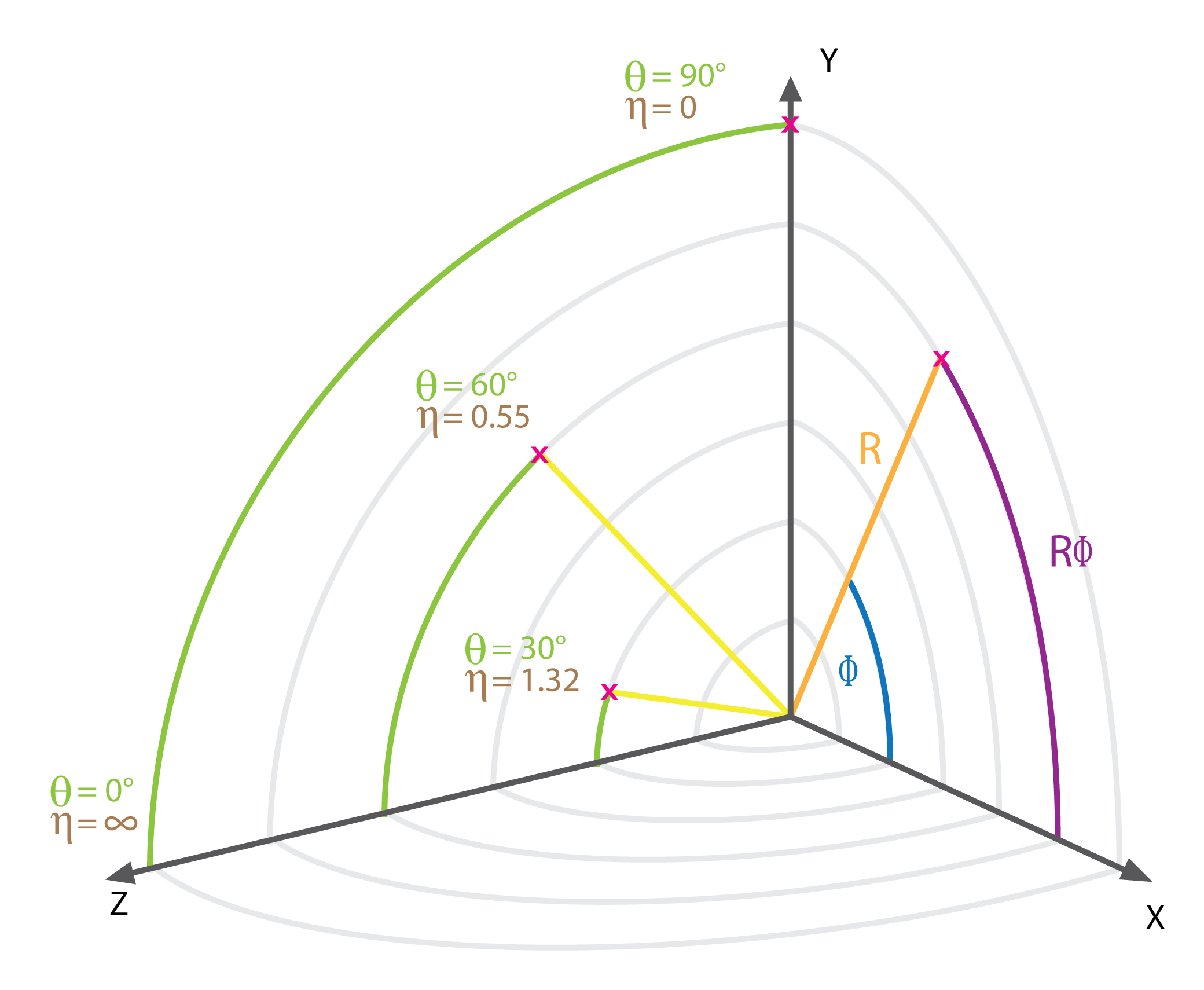
Coordinate conventions

Per convention, the z axis points along the beam axis, the y axis upwards and the x axis horizontal towards the LHC centre. Furthermore, the azimuthal angle \phi, which describes the angle in the x - y plane, the polar angle \theta, which describes the angle in the y - z plane and the pseudorapidity \eta, which is defined as $\eta = -ln\left(tan\frac{\theta}{2}\right)$ are introduced. The coordinates are visualised in [@fig:cmscoords].

{#fig:cmscoords width=60%}

The tracking system

The tracking system is built of two parts, first a pixel detector and then silicon strip sensors. It is used to reconstruct the tracks of charged particles, measuring their charge sign, direction and momentum. It is as close to the collision as possible to be able to identify secondary vertices.

The electromagnetic calorimeter

The electromagnetic calorimeter measures the energy of photons and electrons. It is made of tungstate crystal. When passed by particles, it produces light in proportion to the particle's energy. This light is measured by photodetectors that convert this scintillation light to an electrical signal. To measure a particles energy, it has to leave its whole energy in the ECAL, which is true for photons and electrons, but not for other particles such as hadrons (particles formed of quarks) and muons. They too leave some energy in the ECAL.

The hadronic calorimeter

The hadronic calorimeter (HCAL) is used to detect high energy hadronic particles. It surrounds the ECAL and is made of alternating layers of active and absorber material. While the absorber material with its high density causes the hadrons to shower, the active material then detects those showers and measures their energy, similar to how the ECAL works.

The solenoid

The solenoid, giving the detector its name, is one of the most important feature. It creates a magnetic field of 3.8 T and therefore makes it possible to measure momentum of charged particles by bending their tracks.

The muon system

Outside of the solenoid there is only the muon system. It consists of three types of gas detectors, the drift tubes, cathode strip chambers and resistive plate chambers. The system is divided into a barrel part and two endcaps. Together they cover 0 < |\eta| < 2.4. The muons are the only detected particles, that can pass all the other systems without a significant energy loss.

The Particle Flow algorithm

The particle flow algorithm is used to identify and reconstruct all the particles arising from the proton - proton collision by using all the information available from the different sub-detectors of the CMS. It does so by extrapolating the tracks through the different calorimeters and associating clusters they cross with them. The set of the track and its clusters is then no more used for the detection of other particles. This is first done for muons and then for charged hadrons, so a muon can't give rise to a wrongly identified charged hadron. Due to Bremsstrahlung photon emission, electrons are harder to reconstruct, for them a specific track reconstruction algorithm is used [TODO]. After identifying charged hadrons, muons and electrons, all remaining clusters within the HCAL correspond to neutral hadrons and within ECAL to photons. If the list of particles and their corresponding deposits is established, it can be used to determine the particles four momentums. From that, the missing transverse energy can be calculated and tau particles can be reconstructed by their decay products.

Jet clustering

Because of the hadronisation it is not possible to uniquely identify the originating particle of a jet. Nonetheless, several algorithms exist to help with this problem. The algorithm used in this thesis is the anti-k_t clustering algorithm. It arises from a generalization of several other clustering algorithms, namely the k_t, Cambridge/Aachen and SISCone clustering algorithms.

The anti-k_t clustering algorithm associates hard particles with their soft particles surrounding them within a radius R in the \eta - \phi plane forming cone like jets. If two jets overlap, the jets shape is changed according to its hardness. A softer particles jet will change its shape more than a harder particles. A visual comparision of four different clustering algorithms can be seen in [@fig:antiktcomparision].

{#fig:antiktcomparision}

\newpage

Method of analysis

As described in …, an excited quark q* can decay to a quark and any boson. The branching ratios are calculated to be as follows:

The majority of excited quarks will decay to a quark and a gluon, but as this is virtually impossible to distinguish from QCD effects (for example from the qg->qg processes), this analysis will focus on the processes q*->qW and q*->qZ. In this case, due to jet substructure studies, it is possible to establish a discriminator between QCD background and jets originating in a W/Z decay. They still make up roughly 20 % of the signal events to study and therefore seem like a good choice.

To find signal events in the data, this thesis looks at the dijet invariant mass distribution. It is assumed to only consist of QCD background and signal events, other backgrounds are neglected. If the q* particle exists, this distribution should show a peak at its invariant mass. This peak will be looked for with statistical methods explained later on.

Signal/Background modelling

To be able to first make sure the setup is working as intended, simulated samples are of background and signal are used. For that, Monte Carlo simulations are used. The different particle interactions that take in a proton - proton collision are simulated using the probabilities provided by the Standard Model. Later on, also detector effects are applied to make sure, they look like real data coming from the CMS detector. The q* signal samples are simulated by the probabilities given by the q* theory and assuming a cross section of \SI{1}{\per\pico\barn}.

The invariant mass distribution of the QCD background sample is fitted using the following function with three parameters p0, p1, p2: \begin{equation} \frac{dN}{dm_{jj}} = \frac{p_0 \cdot ( 1 - m_{jj} / \sqrt{s} )^{p_2}}{ (m_{jj} / \sqrt{s})^{p_1}} \end{equation} Whereas m_{jj} is the invariant mass of the dijet and p_0 is a normalisation parameter. Two and four parameter functions have also been studied but found to not fit the background as good as this one.

The signal is fitted using a double sided crystal ball function. A gaussian and a poisson have also been studied but found to not fit the signal sample very well.

\newpage

Preselection and data quality

To separate the background from the signal, several cuts have to be introduced. The selection of events is divided in two parts. The first one (the preselection) adds some cuts for trigger efficiency as well as general physics motivated cuts. It is not expected to already provide a good separation of background and signal. In the second part, different taggers will be used as a discriminator between QCD background and signal events. After the preselection, it is made sure, that the simulated samples represent the real data well.

Preselection

From a decaying q* particle, we expect two jets in the endstate. Therefore a cut of number of jets \ge 2 is added. More jets are also possible because of jets originating in QCD effects such as gluon - gluon interactions. The second cut is on \Delta\eta. The q* particle is expected to be very heavy and therefore almost stationary. Its decay products should therefore be close to back to back, which means a low \Delta\eta. To maintain comparability, the same cut as in previous research of \Delta\eta \le 1.3 will be used. The last cut in the preselection is on the dijet invariant mass: m_{jj} \ge \SI{1050}{\giga\eV}. It is important for a high trigger efficiency. To summarise, the following cuts are applied during preselection:

1. Number of jets \ge 2
2. \Delta\eta \le 1.3
3. m_{jj} \ge \SI{1050}{\giga\eV}

Data - Monte Carlo Comparision

To ensure high data quality, the MC QCD background sample is now being compared to the actual data of the corresponding year collected by the CMS detector. This is done for the years 2016, 2017 and 2018. The distributions are normalised on the invariant mass distribution. For most distributions, no significant difference is seen between data and simulation. In 2018, way more events have a high number of primary vertices in the real data than in the simulated sample. This is being investigated by a CMS workgroup already but should not affect this analysis.

Sideband

The sideband is introduced to make sure there are no unwanted side effects of the used cuts. It adds a cut, that makes sure, no data in the sideband is used for the actual analysis. As sideband, the region where the mass of one of the two jets with the highest transverse momentum ($p_t$) is more than 105 GeV. Because the decay of a q* to a vector boson is being investigated, one of the two jets should have a mass between 105 GeV and 35 GeV. Therefore events with jets that are heavier than 105 GeV will not be used for this analysis which makes them a good sideband to use.

Event substructure selection

This selection is responsible for distinguishing between QCD and signal events by using a tagger to identify jets coming from a vector boson. Two different taggers will be used to later compare the results. The decay analysed includes either a W or Z boson, which are, compared to the particles in QCD effects, very heavy. This can be used by adding a cut on the softdropmass of a jet. The softdropmass is calculated by removing wide angle soft particles from the jet to counter the effects of contamination from initial state radiation, underlying event and multiple hadron scattering. The softdropmass of at least one of the two leading jets is expected to be within \SI{35}{\giga\eV} and \SI{105}{\giga\eV}.

N-Subjettiness

The N-subjettiness \tau_n is defined as

\begin{equation} \tau_N = \frac{1}{d_0} \sum_k p_{T,k} \cdot \text{min}{ \Delta R_{1,k}, \Delta R_{2,k}, …, \Delta R_{N,k} } \end{equation}

with k going over the constituent particles in a given jet, p_{T,k} being their transverse momenta and $\Delta R_{J,k} = \sqrt{(\Delta\eta)^2 + (\Delta\phi)^2}$ being the distance of a candidate subjet J and a constituent particle k in the rapidity-azimuth plane. It quantifies to what degree a jet can be regarded as a jet composed of N subjets. It has been shown, that \tau_{21} = \tau_2/\tau_1 is a good discriminator between QCD events and events originating from the decay of a boosted vector boson.

The \tau_{21} cut is applied to the one of the two highest p_t jets passing the softdropmasswindow. If both of them pass, it is applied to the one with higher p_t.

DeepBoosted

The deep boosted tagger uses a trained neural network to identify decays originitating in a vector boson. It is supposed to give better efficiencies than the older N-Subjettiness method.

Optimization

To figure out the best value to cut on the discriminators introduced by the two taggers, a value to quantify how good a cut is has to be introduced. For that, the significance calculated by \frac{S}{\sqrt{B}} will be used. S stands for the amount of signal events and B for the amount of background events in a given interval. This value assumes a gaussian error on the background so it will be calculated for the 2 TeV masspoint where enough background events exist to justify this assumption. The value therefore represents how good the signal can be distinguished from the background in units of the standard deviation of the background. As interval, a 10 % margin around the masspoint is chosen.

As a result, the \tau_{21} cut is placed at \le 0.35 and the VvsQCD cut is placed at \ge 0.83.

\newpage

Signal extraction

Uncertainties

\newpage

Results

2016

previous research

2016 + 2017 + 2018

Summary